Partial Confinement Utilization for Rectangular Concrete Columns Subjected to Biaxial Bending and Axial Compression

Abstract

The prediction of the actual ultimate capacity of confined concrete columns requires partial confinement utilization under eccentric loading. This is attributed to the reduction in compression zone compared to columns under pure axial compression. Modern codes and standards are introducing the need to perform extreme event analysis under static loads. There has been a number of studies that focused on the analysis and testing of concentric columns. On the other hand, the augmentation of compressive strength due to partial confinement has not been treated before. The higher eccentricity causes smaller confined concrete region in compression yielding smaller increase in strength of concrete. Accordingly, the ultimate eccentric confined strength is gradually reduced from the fully confined value f _cc (at zero eccentricity) to the unconfined value $f_{c}^{{\prime }}$ (at infinite eccentricity) as a function of the ratio of compression area to total area of each eccentricity. This approach is used to implement an adaptive Mander model for analyzing eccentrically loaded columns. Generalization of the 3D moment of area approach is implemented based on proportional loading, fiber model and the secant stiffness approach, in an incremental-iterative numerical procedure to achieve the equilibrium path of P–ε and M–φ response up to failure. This numerical analysis is adapted to assess the confining effect in rectangular columns confined with conventional lateral steel. This analysis is validated against experimental data found in the literature showing good correlation to the partial confinement model while rendering the full confinement treatment unsafe.

1 Introduction

It was not until very recently that design specifications and codes of practice, like AASHTO LRFD, started realizing the importance of introducing extreme event load cases that necessitates accounting for advanced behavioral aspects like confinement. Confinement adds other requirements to column analysis as it increases the column’s capacity and ductility. Accordingly, confinement needs special nonlinear analysis to yield accurate predictions. Nevertheless the literature is still lacking specialized analysis tools that take into account partial confinement effects despite the availability of all kinds of concentric confinement models.

Richart et al. (1929) introduced the lateral pressure term in the confined strength equation. From this point on, many concentric models were developed that represented the confined concrete behavior based on tests of plain and reinforced concrete in a form of fractional or exponential functions. Sheikh and Uzumeri (1982) introduced the arching effect between the longitudinal rebars vertically and in between the ties horizontally. Many parameters such as tie spacing and arrangement, column shape, concrete strength were studied thoroughly in various models that followed (Park et al. 1982; Scott et al. 1982; Fafitis and Shah 1985; Mander et al. 1988; Fujii et al. 1988; Saatcioglu and Razvi 1992; Hsu and Hsu 1994; Cusson and Paultre 1995; Wee et al. 1996; Attard and Setunge 1996; Hoshikuma et al. 1997; Razvi and Saatcioglu 1999; Binici 2005; Braga et al. 2006).

Bonet et al. (2006) compared the analytical and numerical algorithms available that calculate the stress integration in circular and rectangular cross sections. They proposed a new method of using Gauss–Legendre quadrature and the modified thick concrete layers parallel to the neutral axis with any orientation. The stress–strain curve suggested for the analysis was the parabola-rectangle from the Eurocode-2 which did not capture the softening zone.

Lejano (2007) extended Kaba and Mahin (1984) fiber Model method to analyse rectangular sections under biaxial loading. The proposed method utilized Bazant’s Endochronic theory and Ciampi’s model for concrete and steel behavior. The proposed method was not sufficiently validated against experimental work.

Cedolin et al. (2008) developed a method of calculating the design interaction diagram for rectangular cross section under biaxial loading based on the moment contour and Bresler Equations. Paultre and Légeron (2008) showed different code limitations in confinement reinforcement requirements. They proposed new equations, using parametric study, for designing the confinement based on concrete curvature demand.

Campione and Minafo (2010) derived new model for high strength concrete confined with steel ties. They confirmed the existence of non-uniform lateral pressure induced by the lateral ties for square columns and the decreasing of the confining pressure in the vertical direction between the ties.

Samani and Attard (2012) modified Attard and Setunge (1996) model to account for higher levels of confinement. They related the fracture energy with increasing confinement up to a confinement ratio of 0.2. Beyond this confinement limit, the fracture energy decreases down to zero due to the dispersed cracking of the concrete in the cross section.

In a relatively recent study, Abd El Fattah et al. (2011) developed a confinement analysis for eccentrically loaded circular columns based on partial confinement treatment, incremental-iterative nonlinear analysis procedure using a fiber model and the secant stiffness approach.

This study is intended to determine the actual ultimate capacity of confined reinforced concrete rectangular columns subjected to eccentric loading to generate the accurate failure envelope based on a modified eccentricity model accounting for partial confinement effects. The analysis is conducted for rectangular columns confined with conventional transverse steel. It is important to note that the present analysis procedure is benchmarked against experimental results to establish its accuracy and reliability.

2 Material Models

2.1 Concrete Model

In the literature, various models were implemented to assess the ultimate confined capacity of columns under concentric axial load. On the other hand, the effect of partial confinement in case of eccentric load (combined axial load and bending moments) is not investigated in any proposed model. Therefore, it is pertinent to relate the strength and ductility of reinforced concrete to the degree of confinement utilization in a new model.

Unlike fully confined columns under pure axial compression, partially confined columns are those subjected to eccentric loading such that the compression zone does not constitute the entire cross section. Accordingly, gradual reduction in confinement levels is anticipated. This is applicable to short (stub) columns with any pattern of ties to be first characterized by a fully confined model then reduced based on the size of the compression zone or the eccentricity engaged.

Mander model is chosen for this study to represent the case of fully confined and unconfined concrete (Mander et al. 1988). This is found to be the most widely accepted model in the literature (Abd El Fattah 2012). The upper extreme curve refers to concentrically loaded confined concrete (zero eccentricity), while the lower extreme one refers to pure bending applied to concrete (infinite eccentricity). In between the two extremes, an infinite number of stress–strain curves can be generated based on the eccentricity, Fig. 1. The higher the eccentricity, the smaller the confined concrete region in compression. Accordingly, the ultimate confined strength is gradually reduced from the fully confined value f _cc to the unconfined value $f_{c}^{{\prime }}$ as a function of the compression area to section area ratio. In addition, the ultimate strain is gradually reduced from the ultimate strain ε _cu for fully confined concrete to the ultimate strain for unconfined concrete (0.003).

Fig. 1

Eccentricity-based confinement proposed here based on Mander Model.

The relationship between the compression area to section area ratio and normalized eccentricity is complicated in case of rectangular cross sections due to the existence of two bending axes. The axial force location with respect to the two axes causes the compression zone to take an irregular shape sometimes if the applied force is not along one of the axes. Hence the relationship between the compression area and the load eccentricity needs more investigation.

The normalized eccentricity is plotted against the compression area to cross sectional area ratio for rectangular cross sections having different aspect ratios (length to width) at the unconfined failure level. The aspect ratios used are 1:1, 2:1, 3:1, and 4:1, as shown in Figs. 2, 3, 4 and 5, with the section width selected to be 20 inches (508 mm). The section was divided into filaments and for each normalized eccentricity the number of filaments in compression is divided by the total number of filaments in the cross section to represent the compression zone ratio. Each curve in every figure represents a specific α angle (tan α = My/Mx) ranging from 0° to 90°. It is seen from these figures that there is an inversely proportional relationship between the normalized eccentricity and compression zone ratio regardless of the α angle considered.

Fig. 2

Normalized eccentricity versus compression zone to total area ratio (aspect ratio 1:1).

Fig. 3

Normalized eccentricity versus compression zone to total area ratio (aspect ratio 2:1).

Fig. 4

Normalized eccentricity versus compression zone to total area ratio (aspect ratio 3:1).

Fig. 5

Normalized eccentricity versus compression zone to total area ratio (aspect ratio 4:1).

In order to find an accurate mathematical expression that relates the compression zone to load eccentricity, the data from Figs. 2, 3, 4 and 5 are re-plotted as scatter points in Fig. 6.

Fig. 6

Cumulative chart for normalized eccentricity against compression zone ratio (all data points).

The best fitting curve for all these points based on the method of least squares reproduces the following equation:

$$ C_{R} = \frac{{0.2 \times \frac{e}{{\sqrt {bh} }} + 0.1}}{{\frac{e}{{\sqrt {bh} }}}} $$

(1)

where C _R refers to compression area to cross sectional area ratio, e is the eccentricity, b and h are the column dimensions.

The equation that defines the peak strength $\overline{{f_{cc} }}$ under eccentric loading as a function of the compression area ratio is proposed here to be:

$$ \overline{{f_{cc} }} = \frac{1}{{1 + \frac{1}{{C_{R} - 0.2}}}}f_{cc} + \frac{1}{{0.8 + C_{R} }}f_{c}^{\prime} $$

(2)

where $\overline{{f_{cc} }}$ is the peak strength at the eccentricity (e). The first extreme in Eq. (1) is the case of full confinement (e = 0, C _R  = ∞). This makes $\overline{{f_{cc} }}$ in Eq. (2) converge to $f_{cc} .$ The other extreme in Eq. (1) is the case of residual confinement (e = ∞, C _R  = 0.2). This makes $\overline{{f_{cc} }}$ in Eq. (2) converge to $f_{c}^{\prime} .$ In the middle, $\overline{{f_{cc} }}$ is mapped in between the two extremes.

The corresponding strain $\overline{{\varepsilon_{cc} }}$ to the peak strength $\overline{{f_{cc} }} ,$ at the eccentricity (e), is given by

$$ \overline{{\varepsilon_{cc} }} = \varepsilon_{co} \left[ {1 + 5\left( {\frac{{\overline{{f_{cc} }} }}{{f_{c}^{\prime} }} - 1} \right)} \right] $$

(3)

Equation (3) is adapted from the work of Richart et al. (1929) in the case of full confinement and is used for partial confinement stress–strain curve. The maximum strain corresponding to the required eccentricity will be a linear function of stress corresponding to maximum strain for confined concrete f _cu and the maximum unconfined concrete stress f _cuo at ε _cuo  = 0.003, see Fig. 1:

$$ \begin{aligned} \overline{{\varepsilon_{cu} }} & = \overline{{\varepsilon_{cc} }} \left[ {\frac{{\frac{{\overline{{E_{\sec } }} }}{{E_{\sec ,u} }}\bar{r}}}{{\frac{c}{{\overline{{\varepsilon_{cu} }} }} + 1}} - \bar{r} + 1} \right]^{{\frac{1}{{\overline{r} }}}} ,\quad E_{\sec ,u} = \frac{{f_{cu} - f_{cuo} }}{{\varepsilon_{cu} - 0.003}} \\ c & = \frac{{f_{cu} - E_{\sec ,u} \times 0.003}}{{E_{\sec ,u} }} \\ \overline{{E_{\sec } }} & = \frac{{\overline{{f_{cc} }} }}{{\overline{{\varepsilon_{cc} }} }}\quad \bar{r} = \frac{{E_{c} }}{{E_{c} - \overline{{E_{\sec } }} }} \\ \end{aligned} $$

(4)

Equation (4) is derived here to solve for the point of intersection of the stress–strain curve of partial confinement (Eq. (5)) and the line connecting the ultimate confined and the ultimate unconfined points, see Fig. 1.

Any point on the generated curves of the eccentric stress–strain functions can be calculated using the following equation:

$$ f_{c} = \frac{{\overline{{f_{cc} }} \bar{r}\bar{x}}}{{\bar{r} - 1 + \bar{x}^{{\bar{r}}} }} $$

(5)

where

$$ \bar{x} = \frac{{\varepsilon_{c} }}{{\overline{{\varepsilon_{cc} }} }} $$

(6)

$$ \bar{r} = \frac{{E_{c} }}{{E_{c} - \overline{{E_{\sec } }} }} $$

(7)

$$ \overline{{E_{\sec } }} = \frac{{\overline{{f_{cc} }} }}{{\overline{{\varepsilon_{cc} }} }} $$

(8)

Equation (5) is adapted from the work of Mander et al. (1988) in the case of full confinement and used for partial confinement stress–strain curve.

2.2 Steel Model

Steel is assumed to be elastic up to the yield stress then perfectly plastic as shown in Fig. 7.

Fig. 7

Steel stress–strain model.

3 Confined Concrete Concentric Analysis

The concentric axial confined strength f _cc is determined based on the multi axial stress state procedure followed by Mander (1983) based on the concrete plasticity model developed by Willam and Warnke (1975) with surface meridian equations for compression C and tension T derived by Elwi and Murray (1979) from the 3D concrete data of Schickert and Winkler (1977). To determine f _cc, a fast converging iterative procedure is devised by Mander (1983) utilizing the two lateral confined pressures f _lx and f _ly found from the confining effects of the transverse steel according to Mander et al. (1988). Once determined, f _cc, is used in the next section to compute the eccentric strength $\overline{{f_{cc} }}$ for each value of eccentricity (e) considered.

4 Confined Concrete Eccentric Analysis

4.1 Analysis Assumptions

The analysis method of the confined concrete utilizes the fiber procedure accounting for the concrete and steel through the concept of 3D generalized moment of area theorem.

The assumptions made in this analysis are:

• 1. There is perfect bond between the longitudinal steel bars and the concrete.

• 2. Strains along the depth of the column are assumed to be distributed linearly.

• 3. Concrete stress in tension is neglected after cracking.

• 4. The section is numerically divided into a finite number of small filaments each of which is assumed to have a constant strain ε _ci and stress f _ci within the filament, see Fig. 8.

  Fig. 8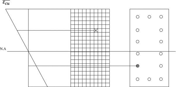

  

  Defining strain for concrete filaments and steel rebars from strain profile.

4.2 The Proposed Method: 3D Generalized Moment of Area Theorem

This approach simulates radial loading of the cross section by keeping the relative proportion between force and moment constant during the loading. Accordingly, all the points comprising an interaction diagram of angle α will be exactly on that 2D interaction diagram. In addition to the ultimate points, the complete load deformation response is generated. The cross section analyzed is loaded incrementally by maintaining a certain eccentricity between the axial force P and the resultant moment M _R . Since M _R is generated as the resultant of M _x and M _y , the angle α = tan⁻¹(M _y /M _x ) is kept constant for a certain 2D interaction diagram. Since increasing the load and resultant moment proportionally causes the neutral axis to vary nonlinearly, the generalized moment of area theorem is devised, Appendix A. This method is based on the general response of rectangular unsymmetrical sections subjected to biaxial bending and axial compression. The asymmetry stems from the different behavior of concrete in compression and tension.

The method is developed using an incremental-iterative analysis algorithm, secant stiffness approach and proportional or radial loading. It is explained in the following steps: Calculating the initial section properties:

• Elastic axial rigidity EA:

  $$ EA = \sum\limits_{i} {E_{c} w_{i} t_{i} } + \sum\limits_{i} {(E_{s} - E_{c} )A_{si} } $$

  (9)

  E _c is the initial modulus of elasticity of the concrete and E _s is the initial modulus of elasticity of the steel bar.

• The depth of the elastic centroid position from the bottom fiber of the section Y _c and from the left side of the section X _c :

  $$ Y_{c} = \frac{{\sum\nolimits_{i} {E_{c} w_{i} t_{i} (H - Y_{i} ) + } \sum\nolimits_{i} {(E_{s} - E_{c} )A_{si} (H - Y_{si} )} }}{EA} $$

  (10)
  $$ X_{c} = \frac{{\sum\nolimits_{i} {E_{c} w_{i} t_{i} (B - X_{i} )} + \sum\nolimits_{i} {(E_{s} - E_{c} )A_{si} (B - X_{si} )} }}{EA} $$

  (11)

  where Y _i and Y _si are measured to the top extreme fiber, X _i and X _si are measured to the right most extreme fiber, see Fig. 9.

  Fig. 9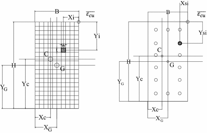

  

  Geometric properties of concrete filaments and steel bars with respect to, geometric centroid and inelastic centroid.

• Elastic flexural rigidity about the elastic centroid EI:

  $$ EI_{x} = \sum\limits_{i} {E_{c} w_{i} t_{i} (H - Y_{i} - Y_{c} )^{2} } + \sum\limits_{i} {(E_{s} - E_{c} )A_{si} } (H - Y_{si} - Y_{c} )^{2} $$

  (12)
  $$ EI_{y} = \sum\limits_{i} {E_{c} } w_{i} t_{i} (B - X_{i} - X_{c} )^{2} + \sum\limits_{i} {(E_{s} } - E_{c} )A_{si} (B - X_{si} - X_{c} )^{2} $$

  (13)
  $$ EI_{xy} = \sum\limits_{i} {E_{c} } w_{i} t_{i} (H - Y_{i} - Y_{c} )\left( {B - X_{i} - X_{c} } \right) + \sum\limits_{i} {(E_{s} } - E_{c} )A_{si} (H - Y_{si} - Y_{c} )\left( {B - X_{si} - X_{c} } \right) $$

  (14)

Typically the initial elastic Y _c  = H/2, X _c  = B/2 and EI _xy  = 0

The depth of the geometric section centroid position from the bottom and left fibers of the section Y _G , X _G :

$$ Y_{G} = \frac{H}{2} $$

(15)

$$ X_{G} = \frac{B}{2} $$

(16)

Performing the incremental-iterative procedure:

• 1. Defining the eccentricity e that specifies the radial path of loading on the interaction diagram. Also, defining the angle α in between the resultant moment GM _R and GM _X , see Fig. 10.

  Fig. 10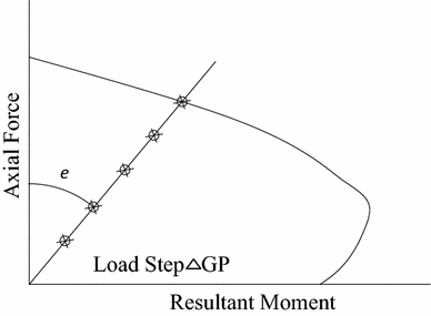

  

  Radial loading concept.

• 2. Defining the loading step ΔGP as a small portion of the maximum load, and computing the axial force at the geometric centroid, see Fig. 10.

  $$ GP_{new} = GP_{old} + \Delta GP $$

  (17)

• 3. Calculating the moment GM _R about the geometric centroid.

  $$ e = \frac{{GM_{R} }}{GP}\quad GM_{R} = e \times GP $$

  (18)
  $$ GM_{X} = GM_{R} \cos \alpha $$

  (19)
  $$ GM_{Y} = GM_{X} \tan \alpha $$

  (20)

• 4. Transferring the moments to the inelastic centroid and calculating the new transferred moments TM _X and TM _Y , Fig. 11:

  $$ TM_{X} = GM_{X} + GP(Y_{G} - Y_{c} ) $$

  (21)
  $$ TM_{Y} = GM_{Y} + GP(X_{G} - X_{c} ) $$

  (22)

  Fig. 11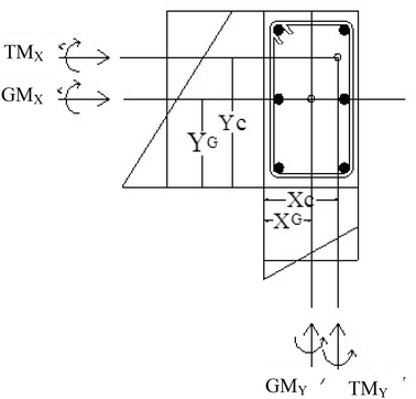

  

  Moment transferring from geometric centroid to inelastic centroid.

  The advantage of transferring the moment to the position of the inelastic centroid is to eliminate the coupling effect between the force and the two moments, since $EAM_{X} = EAM_{Y} = 0$ about the inelastic centroid (Rasheed and Dinno 1994)

  $$ \left[ {\begin{array}{*{20}c} P \\ {TM_{X} } \\ {TM_{Y} } \\ \end{array} } \right] = \left[ {\begin{array}{*{20}c} {EA} & 0 & 0 \\ 0 & {EI_{X} } & {EI_{XY} } \\ 0 & {EI_{XY} } & {EI_{Y} } \\ \end{array} } \right]\left[ {\begin{array}{*{20}c} {\varepsilon_{o} } \\ {\phi_{X} } \\ {\phi_{Y} } \\ \end{array} } \right] $$

  (23)

• 5. Finding: Curvatures ϕ x and ϕ _Y

  $$ \phi_{X} = \frac{{TM_{X} }}{{\beta^{2} }}*EI_{Y} - \frac{{TM_{Y} }}{{\beta^{2} }}*EI_{XY} $$

  (24)
  $$ \phi_{Y} = \frac{{TM_{Y} }}{{\beta^{2} }}*EI_{X} - \frac{{TM_{X} }}{{\beta^{2} }}*EI_{XY} $$

  (25)
  $$ \beta^{2} = EI_{X} EI_{Y} - EI_{xy}^{2} $$

  (26)

• 6. Finding the strain at the inelastic centroid ε _o , the extreme compression fiber strain ε _ec , and the strain at the extreme level of steel in tension ε _es are determined as follow:

  $$ \varepsilon_{o} = \frac{GP}{EA} $$

  (27)
  $$ \varepsilon_{ec} = \varepsilon_{o} + \phi_{X} (H - Y_{c} ) + \phi_{Y} (B - X_{c} ) $$

  (28)
  $$ \varepsilon_{es} = \varepsilon_{o} - \phi_{X} (Y_{c} - Cover) - \phi_{Y} (X_{c} - Cover) $$

  (29)

  Where cover is up to center of the bars

• 7. Calculating strain ε _ci and corresponding stress f _ci in each filament of concrete section by using the Eccentric-Based Model (Eqs. (1)–(8)):

  $$ \begin{aligned} \varepsilon_{ci} & = \frac{GP}{EA} + \frac{{TM_{X} \left( {H - Y_{c} - Y_{i} } \right)}}{{\beta^{2} }}EI_{Y} + \frac{{TM_{Y} \left( {B - X_{c} - X_{i} } \right)}}{{\beta^{2} }}EI_{X} - \frac{{TM_{X} \left( {B - X_{c} - X_{i} } \right)}}{{\beta^{2} }}EI_{XY} \\ & \quad - \frac{{TM_{Y} \left( {H - Y_{c} - Y_{i} } \right)}}{{\beta^{2} }}EI_{XY} \\ \end{aligned} $$

  (30)

• 8. Calculating strain ε _si and corresponding stress f _si in each bar in the given section by using the steel model shown in Fig. 7.

  $$ \begin{aligned} \varepsilon_{si} & = \frac{GP}{EA} + \frac{{TM_{X} \left( {H - Y_{c} - Y_{si} } \right)}}{{\beta^{2} }}EI_{Y} + \frac{{TM_{Y} \left( {B - X_{c} - X_{si} } \right)}}{{\beta^{2} }}EI_{X} - \frac{{TM_{X} \left( {B - X_{c} - X_{si} } \right)}}{{\beta^{2} }}EI_{XY} \\ & \quad - \frac{{TM_{Y} \left( {H - Y_{c} - Y_{si} } \right)}}{{\beta^{2} }}EI_{XY} \\ \end{aligned} $$

  (31)

• 9. Calculating the new section properties: axial rigidity EA, flexural rigidities about the inelastic centroid EI _X , EI _Y , EI _XY , moment of axial rigidity about inelastic centroid EAM _X , EAM _Y , internal axial force F _Z , internal bending moments about the inelastic centroid M _OX , M _OY :

  $$ EA = \sum\limits_{i} {E_{ci} } w_{i} t_{i} + \sum\limits_{i} {(E_{si} - E_{ci} )A_{si} } $$

  (32)
  $$ EAM_{X} = \sum\limits_{i} {E_{ci} } w_{i} t_{i} (H - Y_{c} - \mathop {Y_{i} }\limits^{{}} ) + \sum\limits_{i} {(E_{si} } - E_{ci} )A_{si} (H - Y_{c} - Y_{si} ) $$

  (33)
  $$ EAM_{Y} = \sum\limits_{i} {E_{ci} } w_{i} t_{i} (B - X_{c} - \mathop {X_{i} }\limits^{{}} ) + \sum\limits_{i} {(E_{si} } - E_{ci} )A_{si} (B - X_{c} - X_{si} ) $$

  (34)
  $$ F_{Z} = \sum {f_{ci} w_{i} t_{i} } + \sum {(f_{si} - f_{ci} )A_{si} } $$

  (35)
  $$ EI_{X} = \sum\limits_{i} {E_{ci} } w_{i} t_{i} (H - Y_{c} - Y_{i} )^{2} + \sum\limits_{i} {(E_{si} } - E_{ci} )A_{si} (H - Y_{c} - Y_{si} )^{2} $$

  (36)
  $$ EI_{Y} = \sum\limits_{i} {E_{ci} } w_{i} t_{i} (B - X_{c} - X_{i} )^{2} + \sum\limits_{i} {(E_{si} } - E_{ci} )A_{si} (B - X_{c} - X_{si} )^{2} $$

  (37)
  $$ \begin{aligned} EI_{XY} & = \sum\limits_{i} {E_{ci} } w_{i} t_{i} (H - Y_{c} - Y_{i} )\left( {B - X_{c} - X_{i} } \right) \\ & \quad + \sum\limits_{i} {(E_{si} } - E_{ci} )A_{si} (H - Y_{c} - Y_{si} )\left( {B - X_{c} - X_{si} } \right) \\ \end{aligned} $$

  (38)
  $$ M_{OX} = \sum\limits_{i} {f_{ci} } w_{i} t_{i} (H - Y_{c} - Y_{i} ) + \sum\limits_{i} {(f_{si} } - f_{ci} )A_{si} \left( {H - Y_{c} - Y_{si} } \right) $$

  (39)
  $$ M_{OY} = \sum\limits_{i} {f_{ci} } w_{i} t_{i} (B - X_{c} - X_{i} ) + \sum\limits_{i} {(f_{si} } - f_{ci} )A_{si} \left( {B - X_{c} - X_{si} } \right) $$

  (40)

  where E _ci  = secant modulus of elasticity of the concrete filament = $\frac{{f_{ci} }}{{\varepsilon_{ci} }}.$ and E _si  = secant modulus of elasticity of the steel bar = $\frac{{f_{si} }}{{\varepsilon_{si} }}.$

• 10. Transferring back to the internal moment about the geometric centroid, Fig. 11:

  $$ GM_{OX} = M_{OX} - GP(Y_{G} - Y_{c} ) $$

  (41)
  $$ GM_{OY} = M_{OY} - GP(X_{G} - X_{c} ) $$

  (42)

• 11. Checking the convergence of the inelastic centroid

  $$ TOL_{x} = EAM_{X} /EA/Y_{c} $$

  (43)
  $$ TOL_{y} = EAM_{Y} /EA/X_{c} $$

  (44)

• 12. Comparing the internal force to applied force, internal moments to applied moments, and making sure the moments are calculated about the geometric centroid:

  $$ \left| {GP - F_{Z} } \right| \le 1 \times 10^{ - 5} $$

  (45)
  $$ \left| {GM_{X} - GM_{OX} } \right| \le 1 \times 10^{ - 5} \quad \left| {GM_{Y} - GM_{OY} } \right| \le 1 \times 10^{ - 5} $$

  (46)
  $$ \left| {TOL_{x} } \right| \le 1 \times 10^{ - 5} \quad \left| {TOL_{y} } \right| \le 1 \times 10^{ - 5} $$

  (47)

  If Eqs. (45), (46) and (47) are not satisfied, the location of the inelastic centroid is updated by adding EAM _X /EA and EAM _Y /EA and repeating steps 5–12 till Eqs. (45)–(47) are satisfied.

  $$ Y_{{c_{new} }} = Y_{{c_{old} }} + \frac{{EAM_{X} }}{EA} $$

  (48)
  $$ X_{{c_{new} }} = X_{{c_{old} }} + \frac{{EAM_{Y} }}{EA} $$

  (49)

  Once equilibrium is achieved, the algorithm checks for ultimate strain in concrete ε _ec and steel ε _es not to exceed $\overline{{\varepsilon_{cu} }}$ and 0.05, respectively. Then it increases the loading by ΔGP and runs the analysis again for the new load level using the latest section properties, Fig. 12. Otherwise, if ε _ec equals $\overline{{\varepsilon_{cu} }}$ or ε _es equals 0.05, the target force and resultant moment are recorded as a point on the failure surface for the amount of eccentricity and angle α used.

  Fig. 12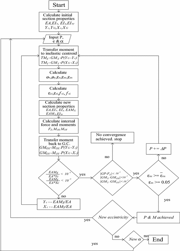

  

  Flowchart of generalized moment of area method used for confined analysis.

5 Results and Discussion

The present simulation procedure is capable of generating column interaction diagrams for eccentric confined compression analysis. For the sake of benchmarking and verifying the accuracy of the present algorithm, the interaction diagrams generated, using the proposed method, are compared with experimental data.

For the sake of comparison, the proposed method is used in generating interaction diagrams using (i) Eq. (2) that accounts for compression zone ratio and (ii) using the following equation directly in terms of the eccentricity (Abd El Fattah et al. 2011):

$$ \overline{{f_{cc} }} = \frac{1}{{1 + \frac{e}{{\sqrt {bh} }}}}\,f_{cc} + \frac{1}{{1 + \frac{{\sqrt {bh} }}{e}}}\;f_{c}^{\prime} $$

(50)

where b and h are the cross section width and height.

The proposed model is compared with eight experimental load cases from the literature as well as with the predictions of Eq. (50) when replacing Eq. (2):

• Case 1 Two experimental data points by Saatcioglu et al. (1995), which has the following column properties: Section Height = 210 mm (8.27 in.), Section Width = 210 mm (8.27 in.), Clear Cover = 13 mm (0.5 in.), Steel Bars in x direction = 3, Steel Bars in y direction = 3, Steel Bar Area = 100 mm² (0.155 in².), Tie Diameter = 9.25 mm (0.364 in.), $f_{c}^{{\prime }}$ = 35.2 MPa (5.1 ksi), f_y = 517 MPa (75 ksi), f_yh = 410 MPa (59.45 ksi), Tie Spacing = 50 mm (1.97 in.), Fig. 13.

  Fig. 13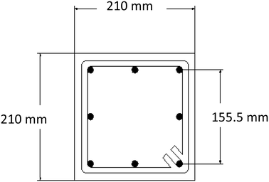

  

  Saatcioglu et al. (1995) Column 1.

  It is evident from Fig. 14 that one of the two points falls perfectly on the proposed interaction diagram while the second point matches the second curve of Eq. (50). The interaction diagram with no eccentricity is un-conservative with respect to both points. It is also worth mentioning that the confinement contribution is significant in this case since the $f_{lmin} /f_{c}^{{\prime }}$ ratio is 12.6%, Table 1.

  Fig. 14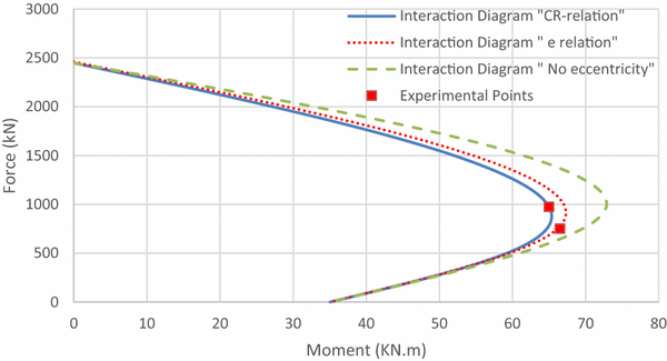

  

  Comparison between different analyses and experimental points of Column 1 (α = 0).

  Table 1 Confinement level measured in terms of $f_{lmin} /f_{c}^{{\prime }}$ for the eight cases considered.

• Case 2 Two experimental data points by Saatcioglu et al. (1995), which has the following column properties: Section Height = 210 mm (8.27 in.), Section Width = 210 mm (8.27 in.), Clear Cover = 13 mm (0.5 in.), Steel Bars in x direction = 4, Steel Bars in y direction = 4, Steel Bar Area = 100 mm² (0.155 in².), Tie Diameter = 9.25 mm (0.364 in.), $f_{c}^{{\prime }}$ = 35.2 MPa (5.1 ksi), f_y = 517 MPa (75 ksi), f_yh = 410 MPa (59.45 ksi), Tie Spacing = 50 mm (1.97 in.), Fig. 15.

  Fig. 15

  

  Saatcioglu et al. (1995) Column 2.

  Figure 16 clearly shows that the two experimental points matches closely the interaction diagram of the proposed Eq. (2) while the solution of Eq. (50) and the case of no partial confinement solution fall outside the two experimental points indicating un-conservative predictions. It is also worth mentioning that the confinement contribution is very significant in this case since the $f_{lmin} /f_{c}^{{\prime }}$ ratio is 22.6%, Table 1.

  Fig. 16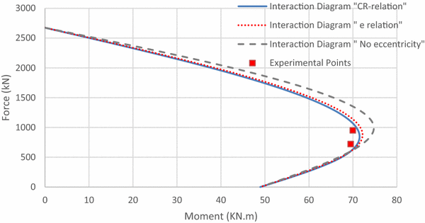

  

  Comparison between different analyses and experimental points of Column 2 (α = 0).

• Case 3 Four experimental data points by Scott et al. (1982), which has the following column properties: Section Height = 450 mm (17.7 in.), Section Width = 450 mm (17.7 in.), Clear Cover = 20 mm (0.787 in.), Steel Bars in x direction = 4, Steel Bars in y direction = 4, Steel Bar Area = 316 mm² (0.49 in².), Tie Diameter = 10 mm (0.394 in.), $f_{c}^{{\prime }}$ = 25.3 MPa (3.67 ksi), f _y  = 435 MPa (63 ksi), f _yh  = 309 MPa (44.8 ksi), Tie Spacing = 72 mm (2.83 in.), Fig. 17.

  Fig. 17

  

  Scott et al. (1982) Column 1.

  It can be seen from Fig. 18 that the four experimental points correlate reasonably well with the interaction diagram of the proposed Eq. (2). It should also be noted that the experimental data points having the same eccentricity but a different strain rate are different. Nevertheless, the inner two points, having a loading strain rate of 0.0000033, are located slightly inside the interaction diagram while the outer two points, representing a higher strain rate of 0.0167, correspond very well with the present envelop curves. It is also worth mentioning that the confinement contribution is noticeable in this case since the $f_{lmin} /f_{c}^{{\prime }}$ ratio is 9.1%, Table 1.

  Fig. 18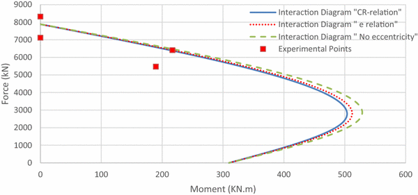

  

  Comparison between different analyses and experimental points of Scott Column 1 (α = 0).

• Case 4 Four experimental data points by Scott et al. (1982), which has the following column properties: Section Height = 450 mm (17.7 in.), Section Width = 450 mm (17.7 in.), Clear Cover = 20 mm (0.787 in.), Steel Bars in x direction = 3, Steel Bars in y direction = 3, Steel Bar Area = 452 mm² (0.7 in².), Tie Diameter = 10 mm (0.394 in.), $f_{c}^{{\prime }}$ = 25.3 MPa (3.67 ksi), f _y  = 394 MPa (57.13 ksi), f _yh  = 309 MPa (44.8 ksi), Tie Spacing = 72 mm (2.83 in.), Fig. 19.

  Fig. 19

  

  Scott et al. (1982) Column 2.

  It can be seen from Fig. 20 that similar observations may be made to those presented by Fig. 18. Since the present analysis assumes static loading, it can be concluded that the strain rate is a parameter that needs further investigation. It is also worth mentioning that the confinement contribution is noticeable in this case since the $f_{lmin} /f_{c}^{{\prime }}$ ratio is 8.8%, Table 1.

  Fig. 20

  

  Comparison between different analyses and experimental points of Scott Column 2 (α = 0).

• Case 5 Five experimental data points by Yoo and Shin. (2007), which has the following two identical column properties: Section Height = 200 mm (7.87 in.), Section Width = 200 mm (7.87 in.), Clear Cover = 20 mm (0.787 in.), Steel Bars in x direction = 2, Steel Bars in y direction = 2, Steel Bar Area = 126.45 mm² (0.196 in².), Tie Diameter = 8.36 mm (0.329 in.), $f_{c}^{{\prime }}$ = 34 MPa (4.931 ksi), f_y = 414 MPa (60 ksi), f_yh = 414 MPa (60 ksi), Tie Spacing = 100 mm (3.3 in.), Fig. 21.

  Fig. 21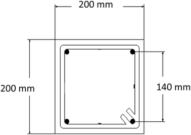

  

  Yoo and Shin (2007) Columns 1–3.

  Figure 22 shows two experimental data points for uniaxial bending (α = 0). It is evident that the near balance and tension controlled points match perfectly the proposed interaction diagram of Eq. (2) while the cases of Eq. (50) and full confinement appear to be un-conservative. Figure 23 presents a comparison against three experimental data points for equi-biaxial bending (α = 45). It is evident from this figure that all three interaction graphs match each other almost exactly indicating minimal partial confinement effects in this case due to the limited confinement effects in general (wide tie spacing), especially for (α = 45) where small number of corner filaments reaches the ultimate confined strength. The three experimental points are close to the balanced point interaction curve. It is also worth mentioning that the confinement contribution in this case is low since the $f_{lmin} /f_{c}^{{\prime }}$ ratio is 4.8%, which is way smaller than the same ratio that causes an ascending second branch in the confined stress–strain response of columns wrapped with FRP (8%), Table 1.

  Fig. 22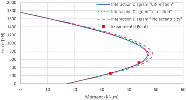

  

  Comparison between different analyses and experimental points of Yoo and Shin Column 1 (α = 0).

  Fig. 23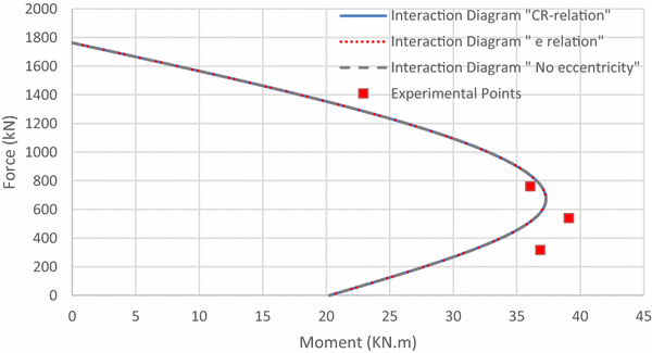

  

  Comparison between different analyses and experimental points of Yoo and Shin Column 1 (α = 45).

• Case 6: Three experimental data points by Yoo and Shin. (2007), which has the following column properties: Section Height = 200 mm (7.87 in.), Section Width = 200 mm (7.87 in.), Clear Cover = 20 mm (0.787 in.), Steel Bars in x direction = 2, Steel Bars in y direction = 2, Steel Bar Area = 126.45 mm² (0.196 in².), Tie Diameter = 8.36 mm (0.329 in.), $f_{c}^{{\prime }}$ = 62 MPa (8.992 ksi), f_y = 414 MPa (60 ksi), f_yh = 414 MPa (60 ksi), Tie Spacing = 100 mm (3.3 in.), Fig. 21.

  Figure 24 illustrates a comparison against three experimental data points for biaxial bending (α = 22.5). It is evident from this figure that all three interaction graphs match closely except near the balanced point indicating small partial confinement effects in this case too. The three experimental points are close to the balanced point interaction curve as well. The only variation of this case from case 5 is the higher $f_{c}^{{\prime }}$ value. It is also worth mentioning that the confinement contribution in this case is very low since the $f_{lmin} /f_{c}^{{\prime }}$ ratio is 2.7%, which is significantly smaller than the same ratio that causes an ascending second branch in the confined stress–strain response of columns wrapped with FRP (8%), Table 1.

  Fig. 24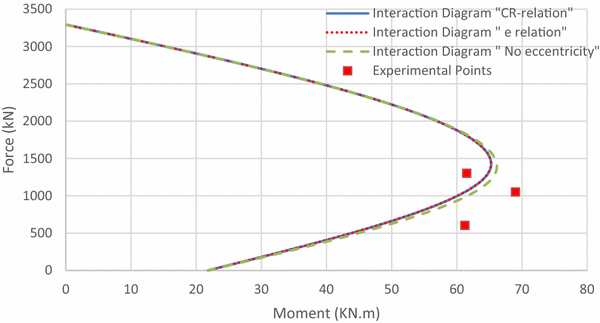

  

  Comparison between different analyses and experimental points of Yoo and Shin Column 2 (α = 22.5).

• Case 7: Three experimental data points by Yoo and Shin. (2007), which has the following column properties: Section Height = 200 mm (7.87 in.), Section Width = 200 mm (7.87 in.), Clear Cover = 20 mm (0.787 in.), Steel Bars in x direction = 2, Steel Bars in y direction = 2, Steel Bar Area = 126.45 mm² (0.196 in².), Tie Diameter = 8.36 mm (0.329 in.), $f_{c}^{{\prime }}$ = 57 MPa (8.26 ksi), f _y  = 414 MPa (60 ksi), f _yh  = 414 MPa (60 ksi), Tie Spacing = 100 mm (3.3 in.), Fig. 21.

  Figure 25 shows a comparison against three experimental data points for equi-biaxial bending (α = 45). It is evident from this figure that all three interaction graphs match each other closely indicating negligible partial confinement effects in this case too. The three experimental points are close enough and just outside the interaction curves that appear to be slightly on the conservative side. The only variation of this case from case 6 is the slightly lower $f_{c}^{{\prime }}$ value. It is also worth mentioning that the confinement contribution in this case is very low since the $f_{lmin} /f_{c}^{{\prime }}$ ratio is 2.9%, which is significantly smaller than the same ratio that causes an ascending second branch in the confined stress–strain response of columns wrapped with FRP (8%), Table 1.

  Fig. 25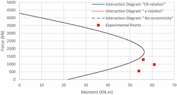

  

  Comparison between different analyses and experimental points of Yoo and Shin Column 3 (α = 45).

• Case 8 Two experimental data points by Zahn et al. (1989), which has the following column properties: Section Height = 400 mm (15.74 in.), Section Width = 400 mm (15.74 in.), Clear Cover = 8 mm (0.31 in.), Steel Bars in x direction = 4, Steel Bars in y direction = 4, Steel Bar Area = 200.6 mm² (0.311 in².), Tie Diameter = 10 mm (0.394 in.), $f_{c}^{{\prime }}$ = 28.8 MPa (4.177 ksi), fy = 423 MPa (61.3 ksi), fyh = 318 MPa (46.1 ksi), Tie Spacing = 65 mm (2.56 in.), Fig. 26.

  Fig. 26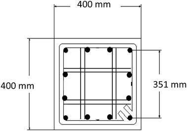

  

  Zahn et al. (1989) Column.

  Figure 27 shows a comparison against two experimental data points for equi-biaxial bending (α = 45). It is evident from this figure that the eccentricity-based interaction graphs match each other closely while the full confinement graph is clearly un-conservative indicating a significant partial confinement effects in this case. The inner experimental point matches the eccentricity-based interaction curves. This point is described by Zahn et al. to correspond to cover spalling while the outer point matching the full confinement curve is said to correspond to column collapse. The significant partial confinement effects in this case is attributed to the use of 4 legs of transverse ties in each of the x and y direction in the column. The confinement contribution in this case is significant since the $f_{lmin} /f_{c}^{{\prime }}$ ratio is 11.4%, which is higher than the same ratio that causes an ascending second branch in the confined stress–strain response of columns wrapped with FRP (8%), Table 1.

  Fig. 27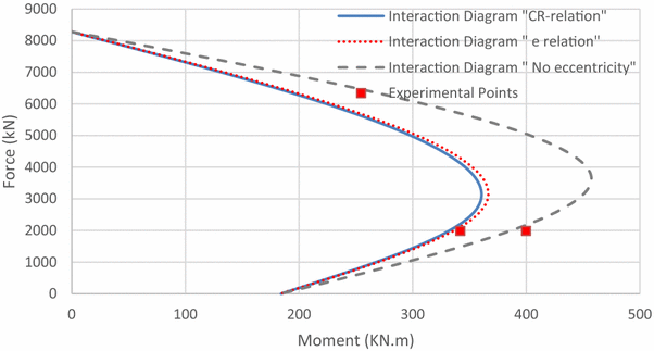

  

  Comparison between different analyses and experimental points of Zahn et al. Column (α = 45).

  It is shown from these figures that the interaction diagrams plotted using Eq. (2), representative of the compression zone area, are the most conservative and accurate in general compared to those of full confinement and those plotted using Eq. (50), a function of eccentricity only. Also the experimental data points correlate well to their corresponding interaction diagrams.

6 Conclusions

In this study, a partial confinement model is developed for rectangular reinforced concrete column sections under general eccentric loading. The model realizes an inverse correlation between the compression zone to the entire section ratio and the eccentricity of the axial compression force due to biaxial moment resultant. Accordingly, the partially confined strength of eccentric loading is morphed between the fully confined case under pure axial compression and the unconfined case under pure bending. Therefore, incrementing the resultant moment and the axial compression takes place proportionally through radial loading to sustain constant eccentricity throughout the loading until failure. The uniaxial moment–axial compression versus uniaxial curvature–axial strain relationship is extended, within the framework of the moment of area concept, from a 2 × 2 to a 3 × 3 stiffness matrix in the case of biaxial bending. The non-linear numerical procedure introduced successfully-predicted the confined capacity of rectangular reinforced concrete columns. The generalized moment of area concept is benchmarked against experimental data, to verify its reliability in providing accurate predictions. The partial confinement effects were shown to be significant or negligible based on the level of transverse steel confinement in the section, which can measured through the ($f_{lmin} /f_{c}^{{\prime }}$) ratio.

References

Abd El Fattah, A. M. (2012). Behavior of concrete columns under various confinement effects. Ph.D. Dissertation, Kansas State University.
Abd El Fattah, A. M., Rasheed, H. A., & Esmaeily, A. (2011). A new eccentricity-based simulation to generate ultimate confined interaction diagrams for circular concrete columns. Journal of the Franklin Institute—Engineering and Applied Mathematics, 348(7), 1163–1176.
Attard, M. M., & Setunge, S. (1996). Stress–strain relationship of confined and unconfined concrete. ACI Materials Journal, 93(5), 432–442.
Binici, B. (2005). An analytical model for stress–strain behavior of confined concrete. Engineering Structures, 27(7), 1040–1051.
Bonet, J. L., Barros, F. M., & Romero, M. L. (2006). Comparative study of analytical and numerical algorithms for designing reinforced concrete section under biaxial bending. Computers & Structures, 84(31–32), 2184–2193.
Braga, F., Gigliotti, R., & Laterza, M. (2006). Analytical stress-strain relationship for concrete confined by steel stirrups and/or FRP jackets. Journal of Structural Engineering, 132(9), 1402–1416.
Campione, G., & Minafo, G. (2010). Compressive behavior of short high-strength concrete columns. Engineering Structures, 32(9), 2755–2766.
Cedolin, L., Cusatis, G., Eccheli, S., & Roveda, M. (2008). Capacity of rectangular cross sections under biaxially eccentric loads. ACI Structural Journal, 105(2), 215–224.
Cusson, D., & Paultre, P. (1995). Stress–strain model for confined high-strength concrete. ASCE Journal of Structural Engineering, 121(3), 468–477.
Elwi, A., & Murray, D. W. (1979). A 3D hypoelastic concrete constitutive relationship. Journal of Engineering Mechanics, 105, 623–641.
Fafitis, A., & Shah, S. P. (1985). Lateral reinforcement for high-strength concrete columns. ACI Special Publication, SP 87-12, pp. 213-232. Detroit, MI: American Concrete Institute.
Fujii, M., Kobayashi, K., Miyagawa, T., Inoue, S., & Matsumoto, T. (1988). A study on the application of a stress–strain relation of confined concrete. In Proceedings of JCA cement and concrete (Vol. 42). Tokyo, Japan: Japan Cement Association.
Hoshikuma, J., Kawashima, K., Nagaya, K., & Taylor, A. W. (1997). Stress–strain model for confined reinforced concrete in bridge piers. Journal of Structural Engineering, 123(5), 624–633.
Hsu, L. S., & Hsu, C. T. T. (1994). Complete stress–strain behavior of high-strength concrete under compression. Magazine of Concrete Research, 46(169), 301–312.
Kaba, S. A., & Mahin, S. A. (1984). Refined modeling of reinforced concrete columns for seismic analysis. Report No. UBC/EERC-84/3. Berkeley, CA: University of California, Berkeley.
Lejano, B. A. (2007). Investigation of biaxial bending of reinforced concrete columns through fiber method modeling. Journal of Research in Science, Computing, and Engineering, 4(3), 61–73.
Mander, J. B. (1983). Seismic design of bridge piers. Ph.D. Thesis, University of Canterbury, Christchurch, New Zealand.
Mander, J. B., Priestley, M. J. N., & Park, R. (1988). Theoretical stress–strain model for confined concrete. Journal of Structural Engineering, ASCE, 114(8), 1827–1849.
Park, R., Priestley, M. J. N., & Gill, W. D. (1982). Ductility of square confined concrete columns. Journal of Structural Division, ASCE, 108(ST4), 929–950.
Paultre, P., & Légeron, F. (2008). Confinement reinforcement design for reinforced concrete columns. Journal of Structural Engineering, ASCE, 134(5), 738–749.
Rasheed, H. A., & Dinno, K. S. (1994). An efficient nonlinear analysis of RC sections. Computers & Structures, 53(3), 613–623.
Razvi, S., & Saatcioglu, M. (1999). Confinement model for high-strength concrete. Journal of Structural Engineering, 125(3), 281–289.
Richart. F. E., Brandtzaeg, A., & Brown, R. L. (1929). The failure of plain and spirally reinforced concrete in compression. Bulletin No. 190, Engineering Station. Urbana, IL: University of Illinois.
Saatcioglu, M., & Razvi, S. R. (1992). Strength and ductility of confined concrete. Journal of Structural Engineering, 118(6), 1590–1607.
Saatcioglu, M., Salamt, A. H., & Razvi, S. R. (1995). Confined columns under eccentric loading. Journal of Structural Engineering, 121(11), 1547–1556.
Samani, A. K., & Attard, M. (2012). A stress–strain model for uniaxial and confined concrete under compression. Engineering Structures, 41, 335–349.
Schickert, G., & Winkler, H. (1977). Results of tests concerning strength and strain of concrete subjected to multiaxial compressive stresses (p. 277). No: Deutscher Ausschuss for Stahlbeton (Berlin).
Scott, B. D., Park, R., & Priestley, N. (1982). Stress–strain behavior of concrete confined by overlapping hoops at law and high strain rates. ACI Journal, 79(1), 13–27.
Sheikh, S. A., & Uzumeri, S. M. (1982). Analytical model for concrete confinement in tied columns. Journal of Structural Engineering, ASCE, 108(ST12), 2703–2722.
Wee, T. H., Chin, M. S., & Mansur, M. A. (1996). Stress–strain relationship of high strength concrete in compression. Journal of Materials in Civil Engineering, 8(2), 70–76.
Willam, K. J., & Warnke, E. P. (1975). Constitutive model for the triaxial behavior of concrete. The International Association for Bridge and Structural Engineering, 19, 1–31.
Yoo, S. H., & Shin, S. W. (2007). Variation of ultimate concrete strain at RC columns subjected to axial loads with bi-directional eccentricities. Key Engineering Materials, 348–349, 617–620.
Zahn, F., Park, R., & Priestley, M. J. N. (1989). Strength and ductility of square reinforced concrete column sections subjected to biaxial bending. ACI Structural Journal, 86(2), 123–131.
Acknowledgements
This work was developed under a research project KTRAN KSU-10-06 funded by the Kansas Department of Transportation. The encouragement and support of Kenneth Hurst and John Jones is highly acknowledged.
Author information
Authors and Affiliations
Corresponding author
Rights and permissions
Open Access This article is distributed under the terms of the Creative Commons Attribution 4.0 International License (http://creativecommons.org/licenses/by/4.0/), which permits unrestricted use, distribution, and reproduction in any medium, provided you give appropriate credit to the original author(s) and the source, provide a link to the Creative Commons license, and indicate if changes were made.
About this article
Cite this article
Abd El Fattah, A.M., Rasheed, H.A. & Al-Rahmani, A.H. Partial Confinement Utilization for Rectangular Concrete Columns Subjected to Biaxial Bending and Axial Compression. Int J Concr Struct Mater 11, 135–149 (2017). https://doi.org/10.1007/s40069-016-0178-z
Received:
Accepted:
Published:
Issue Date:
DOI: https://doi.org/10.1007/s40069-016-0178-z